Machine Learning Project — Unsupervised Learning and Dimensionality Reduction
1. Abstract
This project will focus on 2 clustering methods in unsupervised learning, 4 dimension reduction techniques, and their performance on the two datasets: loan eligibility and student math performance.
2. Introduction
2 clustering methods to be tested and compared:
- k-means clustering
- Expectation Maximization
4 dimensionality reduction algorithms:
1. PCA
2. ICA
3. Randomized Projections
4. Tree-based feature selection
For the above algorithms, I will first apply each of them to the two datasets, and then combine one clustering method with one dimensionality reduction algorithm (for each of the above algorithms) to both of the datasets. Then, I will apply the 4 dimensionality reduction algorithms to one of the two datasets and train with the Neural Network model. From there, I will apply the clustering algorithms first to get new data (from clustering), then train with Neural Network mode. The main purpose of the experiment is to explore and compare the performance of these methods, along with comparing with previously implemented models.
3. Dataset
For this project, I selected the following datasets:
- Check Loan Eligibility
- Student Performance (Math only)
The loan eligibility data set is a set of processed data for modeling the eligibility check, based on features like gender, education, income, loan amount, credit history, etc. It consists of 12 columns, of which 10 are integer columns (binary) and 2 are decimal columns. It has a clear y column named Loan_Status (detailed information can be found in the dataset documentation). I have evaluated it from an ethical perspective in another project and it is an interesting data set to evaluate historical biases as well. Therefore, I would like to use it for the ML algorithms and see if different algorithms will induce different biases towards different groups.
The student performance data set was drawn from student achievement in secondary education at two Portuguese schools. The data attributes include student grades, demographic, social, and school-related features (detailed information can be found in the dataset documentation), and it was collected by using school reports and questionnaires. I have only selected the data of the Math subject. The data was specifically modeled under binary/five-level classification and regression tasks. An interesting point about this data set is that it includes three potential y columns: G1, G2, G3, corresponding to 1st, 2nd and 3rd-period grades. However, G2 is dependent on G1, and G3 is dependent on both G1 and G2. I find that it could be useful for Bayesian analysis in the future. Therefore, I would like to use it for this demonstration as it is versatile and easy to implement for multiple models.
4. Method and Individual Analysis
The implementation methods will be briefly introduced in the following section, but many details will be skipped since it is available on sklearn the documentation page. all random_state parameters will be set to 123.
Evaluation methods of the following will be performed (implementation adopted from sklearn.metrics):
- Silhouette Score: determine the degree of separation between clusters
- Adjusted Rand Index: computes a similarity measure between actual labels from the dataset and the predicted labels from the clustering results
- Mutual Information based scores: a function that measures the agreement of the two assignments, ignoring permutations
4.1 k-means Clustering
I selected the implemented algorithm from sklearn.cluster.KMeans, which clusters data by trying to separate samples in n groups of equal variance, minimizing a criterion known as the inertia or within-cluster sum-of-squares (the distance metric here). By default, it uses Lloyd’s algorithm to minimize and re-center. It would only work with numeric values, therefore pre-processing for the datasets is needed.
In the experiment, I aim to find the k value to maximize the adjusted rand index and mutual information-based scores when comparing the cluster results with the known labels. In this way, it would help to indicate the success of clustering on the multiple dimension data sets.
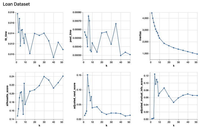
From the above chart, we observe that the fitting time and prediction time for the k-means model does not change much with different k values. As k increases, the inertia of the k-means model keeps decreasing. This says that as k increases, the dataset is worse clustered by K-Means. Therefore, we should choose a smaller k to best fit the dataset. From the bottom two charts, it shows that the best k value to maximize the two scores of interest will be k = 5. From the silhouette chart, it shows that at k = 5, it reaches a local maximum. Therefore, I think the results of the different metrics generally agree with each other.

From the above chart, we observe that the fitting time and prediction time for the k-means model do not change much with different k values for the math dataset either. As k increases, the inertia of the k-means model keeps decreasing. This says that as k increases, the dataset is worse clustered by K-Means. Therefore, we should choose a smaller k to best fit the dataset. From the bottom two charts, it shows that the best k value to maximize the two scores of interest will be k = 4. Based on the silhouette chart, it shows that at k = 4, although it is not a maximum, it is still of high value in the entire chart. Therefore, I think the results of the different metrics generally agree with each other.
4.2 Expectation Maximization
I selected the implemented algorithm from sklearn.mixture, which enables one to learn Gaussian Mixture Models (diagonal, spherical, tied and full covariance matrices supported), sample them, and estimate them from data. I will use the default method covariance_type=full so that each component has its own general covariance matrix. I plan to use init_params=kmeans so that it uses k-means clustering to initialize the weights, the means, and the precisions. It would only work with numeric values, therefore pre-processing for the datasets is needed.

From the above chart, we observe that the fitting time and prediction time for the k-means model does not change much with different k values. From the bottom two charts, it shows that the best n value to maximize the two scores of interest will be n = 4. From the silhouette chart, it shows that at n = 4, it reaches a local maximun. Therefore, I think the results of the different metrics generally agree with each other.

From the above chart, we observe that the best n value to maximize the two scores of interest will be n = 9. From the silhouette chart, it shows that at n = 9, although it is not a maximum, it is still of high value in the entire chart. Therefore, I think the results of the different metrics generally agree with each other.
4.3 PCA
I selected the implemented algorithm from sklearn.decomposition.PCA. It uses linear dimensionality reduction with Singular Value Decomposition of the data to project it to a lower dimensional space. The input data is centered but not scaled for each feature before applying the SVD. We will see the transformed data structure and apply the transformed data to the clustering methods.
In the experiment, I grabbed the variance ratios from different dimensions of the PCA models, and achieved the following plot:
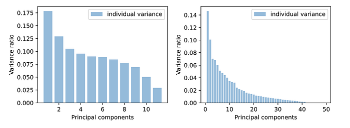
From the above chart, it is observed that the loan dataset (on the left), with 9 features, can cover roughly 90% of the data variance, while for math dataset (on the right), with 30 features, can cover roughly 90% of the data variance. We will keep these numbers to process data for the clustering algorithms.
4.4 ICA
I selected the implemented algorithm from sklearn.decomposition.FastICA. Its purpose is to separate a multivariate signal into additive subcomponents that are maximally independent.
Since there is no good metric to measure the best number of subcomponents to separate out the signals, I will adopt the PCA results for both datasets (9 for loan, 30 for math).
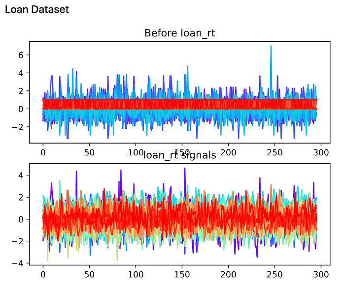
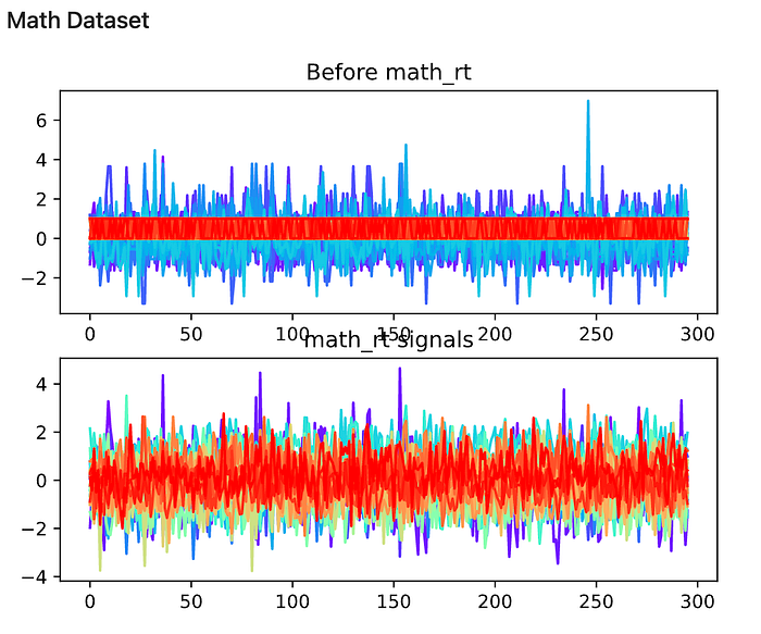
From the experiment, it is observed that the shape of the signals has changed after the ICA transformation. Here I attached the signal chart, colored by different columns of input data.
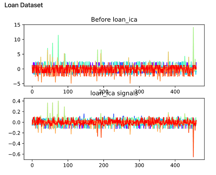
The change is not significant, but it is clear that the variance for each colored line has increased and the boundaries for the lines seem to be set free to increase variance.
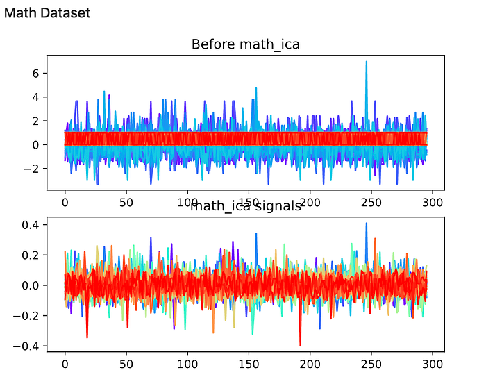
The change here is clear to see: the reddish band in the middle, which represents binary values, is now transformed into a changing line along with other multi-class or numerical data.
4.5 Randomized Projections
I selected the implemented algorithm from sklearn.random_projection. For the same reason as above, I choose to use the PCA results for both datasets (9 for the loan dataset, and 30 for the math dataset) for the number of subcomponents.
From the experiment, it is observed that the shape of the signals changed after the Randomized Projections. Here I attached the signal chart, colored by different columns of input data.
Compared to ICA, both datasets’ values are significantly different from the previous distribution. Especially for the loan dataset, the reddish lines that were binary data are projected better in this model.
4.6 Tree-based feature selection
To implement the algorithm, I referred to the documentation and used both sklearn.ensemble.ExtraTreesClassifier and sklearn.feature_selection.SelectFromModel methods.
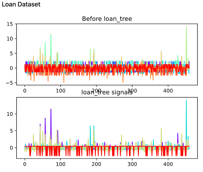
From the experiment, it is observed that the shape of the signals remained roughly the same, only layers have been removed. Here I attached the signal chart, colored by different columns of input data.
Compared to all previous transformations, where the data has been filtered, instead of transformed, based on the relevance to the results. Therefore, we observe a significant color reduction (reduction of feature lines) from the original to the resulting graph, for both of the datasets.

5. Clustering on Datasets of Reduced Dimensions
In the following section, I would show the results of the clustering algorithms on the data sets that were transformed by the above 4 algorithms. In total, 16 analyses will be conducted.
5.1. k-means
Loan Dataset: From the previous k-means experiment, we learn that the best k value to maximize the clustering is: k = 5.

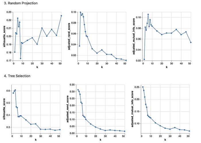
From the above chart, it is observed that the optimal k values have changed:
- PCA: k = 4
- ICA: k = 3
- Random Projection: k = 3
- Tree Selection: k = 2
In addition, compared to the original data and transformed data from PCA and Random Projection, it seems that ICA and Tree Selection have significantly improved the performance of the k-means model. The overall two adjusted rand index scores and mutual information scores have increased to nearly double as high, along with a much larger silhouette score. This suggests that ICA and Tree Selection have effectively removed some noise from the original dataset that might have led to the previously low performance of the k-means model. Especially with the Tree Selection algorithm, the clusters are significantly better grouped together if in the same cluster, and farther away from other groups. Overall, it seems the Tree Selection is the best transformation method here to help optimize the k-means model for the loan dataset.
Math Dataset: From the previous k-means experiment, we learn that the best k value to maximize the clustering is: k = 4.


From the above chart, it is observed that the optimal k values have changed:
- PCA: k = 4 (same as before)
- ICA: k = 25
- Random Projection: k = 10
- Tree Selection: k = 3
In addition, compared to the original data, it seems that PCA, Random Projection and Tree Selection have all slightly improved the silhouette scores. Among them, both Tree Selection and PCA have slightly improved the adjusted rand index scores and mutual information scores, while Random Projection has decreased scores. Overall, it seems that PCA and Tree Selection are good to transform the math dataset to optimize the k-means model.
5.2. Expectation Maximization
Loan Dataset: From the previous EM experiment, we learn that the best n value to maximize the clustering is: n = 4.


From the above chart, it is observed that the optimal n values have changed:
- PCA: n = 6
- ICA: n = 6
- Random Projection: n = 5
- Tree Selection: n = 2
In addition, compared to the original data, it seems that only Tree Selection has significantly improved the silhouette score, the adjusted rand index scores, and the mutual information scores. Under other transformations, the performance of the EM clustering algorithm is even worse than previously. The number of clusters being 2 to best cluster the data points makes a lot of sense since the y data is binary data.
Math Dataset: From the previous EM experiment, we learn that the best n value to maximize the clustering is: n = 9.

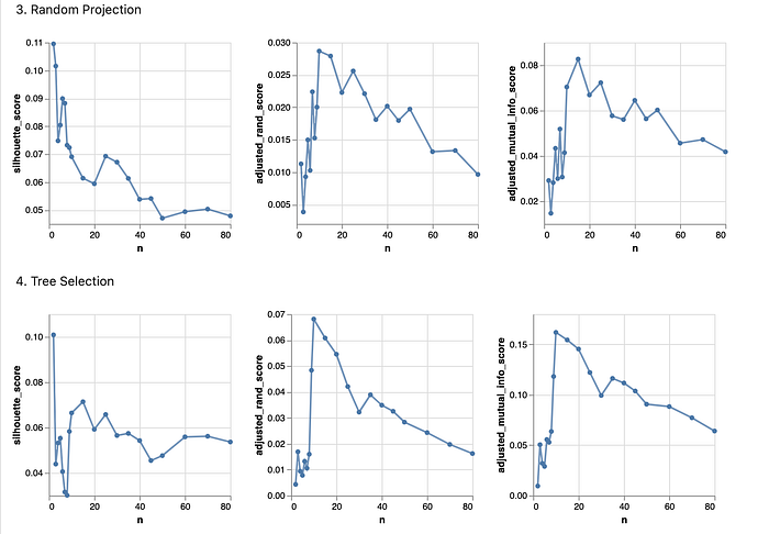
From the above chart, it is observed that the optimal n values have changed:
- PCA: n = 10
- ICA: n = 7
- Random Projection: n = 10
- Tree Selection: n = 10
In addition, compared to the original data, it seems that PCA and Tree Selection have slightly improved the adjusted rand index scores and mutual information scores. Among them, only Tree Selection has a slightly improved silhouette score. Under other transformations, the performance of the EM clustering algorithm is even worse than previously. The number of clusters being 10 to best cluster the data points makes a lot of sense since the y is numerical data that falls into the range of integers (0, 20).
6. Apply PCA-Transformed Loan Dataset to Neural Network Model
Here, I selected the loan dataset that has been transformed with the Tree Selection method to train and test a Neural Network model from assignment 1, and got the following results for accuracy scores:

From the table, we observe that feature selection here seems to improve the accuracy of the Neural Network model. This is when the variance of the features covers 90% of the dataset. I got curious and decided to use a different n = 5 to further shrink the test data. Although it seems to increase the training accuracy, it lowers the test accuracy. However, another factor that might have affected the performance is the StandardScaler() pipeline conducted prior to the feature selection.
7. Neural Network with Clustered PCA-Transformed Loan Dataset
Here, I selected the loan dataset that has been transformed with the PCA method to go through k-means clustering first, and then with the result from the clustering as a new column in the original dataframes, to train and test a Neural Network model from assignment 1, and got the following results for accuracy scores:

From the table, we observe similar behavior with part 6. However, when I got curious and decided to use a different k number (from optimal k = 3 to k = 3), I see an increase in the performance of the Neural Network model. Therefore, I think it proves that the clustering results have a significant impact on the Neural Network model’s performance.
Reference:
Experiment Scripts:
Disclaimer:
This is an adaptation from my school project on Machine Learning class at Georgia Tech.
